DATA for E3SM hybrid modelling
The aim of this project is to develop coarse-scale and data-informed, hybrid methods that produce accurate statistical predictions of climate models. Contemporary climate models run with the resolution needed to capture meteorological events critical to informing decisions for policy makers are computationally too expensive with current computers to capture long timescales. Affordable coarse-scale climate models allow for long timescales to be simulated, but introduce biases owing to the simplified physical process representations at such grid spacings. Historically, decadal scale predictability of catastrophic climate events has relied on the blending of large-scale environments from coarse-scale climate models with high resolution, regionally-confined models. Unfortunately, these methods fail to capture feedback processes between the spatial scales. Hybrid methods hold promise for a new path forward.
The goal of the presented hybrid methodology is to bridge the gap described above. Specifically, we use short-time climate simulations from highly accurate models, in order to machine-learn a correction that is applied to a coarse-scale model. The necessary corrective tendencies are first estimated from a coarse-scale hindcast simulation which is linearly nudged towards a solution derived from a more accurate model. The machine learning (ML) model is trained to predict the nudging tendencies using only the state of the coarse-scale model as inputs. The resulting ML model can then be used in a forecast to apply a corrective tendency to the prognostic state of the atmospheric model at each time step in order to reduce atmospheric model error growth and keep the model evolution on a more realistic manifold.
Climate Model
To test our proposed ML method, we use the E3SM Atmosphere Model (EAM). EAM uses a Spectral Element Dynamical Core coupled to a sophisticated physics parameterizations package and an interactive land surface model (Rasch et al., 2019, Xie et al., 2018). It is the atmospheric component of the coupled Earth system model developed by the U.S. Department of Energy (Golaz et al., 2019). The standard version of EAM uses a 1-degree (100~km) horizontal grid. There are 72 layers in the vertical, extending from the Earth’s surface to about 0.1 hPa (64 km). The key subgrid-scale physical processes considered in EAM include deep convection (Zhang and McFarlane, 1995), turbulence and shallow convection (Golaz et al., 2002, Larson et al., 2002), cloud microphysics (Morrison and Gettelman, 2008, Gettelman et al., 2015, Wang et al., 2014), aerosol life cycle (Liu et al., 2016, Wang et al., 2020), and radiation (Iacono et al., 2008, Mlawer et al., 1997).
In our project, EAM is the target model to be improved with the ML-learn correction. Sea surface temperatures and sea ice extent are prescribed with the observational data from the National Oceanic and Atmospheric Administration (NOAA) Optimum Interpolation (OI) analysis (Reynolds et al., 2002) The external forcings, including volcanic aerosols, solar variability, concentrations of greenhouse gases, and anthropogenic emissions of aerosols and their precursors, were prescribed following the World Climate Research Programme (WCRP) Coupled Model Intercomparison Project Phase 6 (CMIP6) (Eyring et al., 2016, Hoesly et al., 2018, Feng et al., 2020).
The EAM model code for the development of ML model can be found [here].
Nudging Approach
The nudging approach is employed to estimate the biases in EAM’s model state including temperature (T), humidity (Q), zonal wind (U) and meridional wind (V) for the ML training. Here, nudging constrains the model solution of \(\boldsymbol{X}_{m}\) at every grid point toward the reference state of \(\boldsymbol{X}_{\boldsymbol{r}}\) by adding a linear relaxation term to the EAM model equation:
where \(\boldsymbol{X}_{m}\) and \(\boldsymbol{X}_{\boldsymbol{r}}\) refer to the state variables of U, V, T, Q from the EAM predictions and the reference data sets, respectively. The first term on the right-hand side of of the 1st equation represents the effects of large-scale dynamics (e.g. large-scale advection etc.). The second term denotes the parameterized effects of physical processes such as clouds and convection that operate at scales smaller than the model grid and affect the overall dynamics of the system. The third term \(\dot{\boldsymbol{R}}\) is a nudging tendency term that acts as an error correction for \(\boldsymbol{X}_{\boldsymbol{m}}\), calculated as the difference between \(\boldsymbol{X}_{\boldsymbol{m}}\) and \(\boldsymbol{X}_{\boldsymbol{r}}\), scaled by the relaxation time scale \(\tau\) in the 2nd equation.
Pink boxes in Figure 1 illustrate where the nudging-related calculations occur in the default EAM. In a nudged simulation, after the resolved dynamics (see blue box in figure) has been calculated, a nudging tendency term in the form of Eq 2 is calculated for each nudged variable with \(\boldsymbol{X}_{m}\) being the value of $X$ after the dynamical core. After the entire physics parameterization suite has been calculated, the sum of the parameterization-induced tendencies and the nudging tendencies are passed to the physics-dynamics coupling interface.
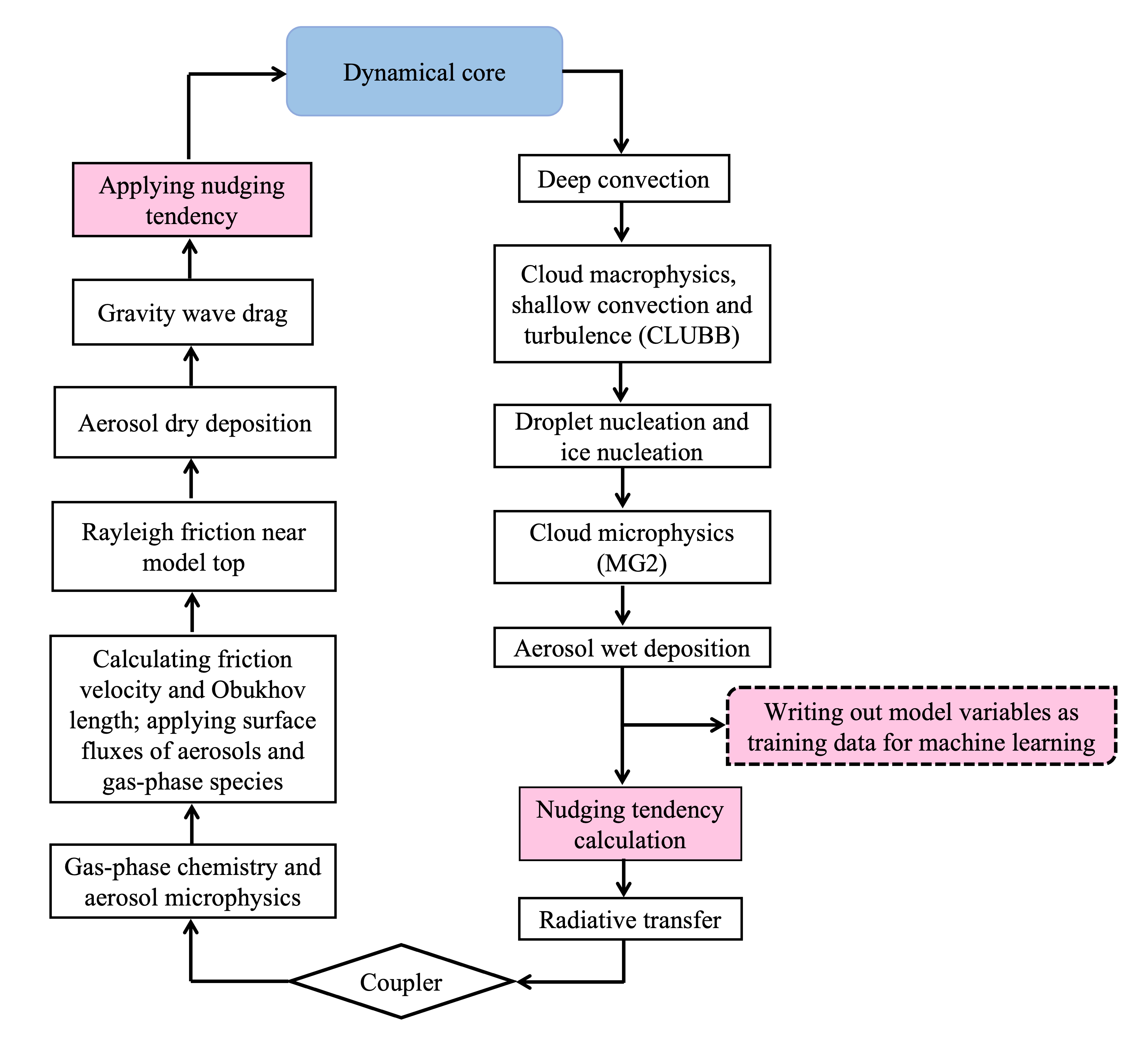
Figure 1: Flowcharts showing the sequence of dynamics and physics calculations within one time step in an EAM simulation. Pink boxes indicate where the nudging-related calculations occur. The calculation of nudging tendency using Eq. (2) occurs before the radiation parameterization.
Nudged training simulation with EAM
In Phase 1, the ML training data are constructed following a “nudge-to-observations” approach described in Watt-Meyer et. al. (2021). In the “nudge-to-observations” approach employed by this project, the observations (i.e. reference data sets) are taken from the ERA5 reanalysis developed by the European Centre for Medium-Range Weather Forecasts (ECMWF) (Hersbach et al., 2020). The raw ERA5 reanalysis data are produced on a \(0.25^{o}\) horizontal grid over the globe, which are spatially remapped to the cubed-sphere grid and the 72 model layers used by EAM, following the method used in the Community Earth System Model Version 2 [CESM2]. Topographical differences between EAM and the reanalysis data are taken into account during the vertical interpolation.
Figure 2a shows the distribution of monthly mean zonal averaged temperature differences between the EAM free-running simulations (CLIM) and ERA5 reanalysis (reference) in January 2010. Most model layers in the Tropics and mid-latitudes exhibit a cold temperature bias. In these regions, the positive temperature nudging tendencies in the nudged simulation act to correct the cold biases (Fig.2b). Generally the time mean nudging tendency removes the systematic “background error” found in the EAM free-running simulations. However, the nudging may not always help to reduce the systematic errors. For example, nudging both wind and temperature can produce a positive tendency of temperature in the northern hemisphere high-latitude (Fig.2b), where the free-running simulations exhibit warm temperature biases, as shown in Fig.2a, suggesting a role of positive feedback that amplifies the upper level temperature biases in the free-running simulations. Using a nudging strategy that constrains humidity in addition to wind and temperature produces rather different nudging tendencies (Fig.2c), revealing the complex relationships between the nudging corrections and the state variables through the nonlinear governing equation (see equation on top of the page). Therefore, we design different nudging strategies to provide an ensemble of nudged simulations with different nudging tendencies and state variables for the ML training.
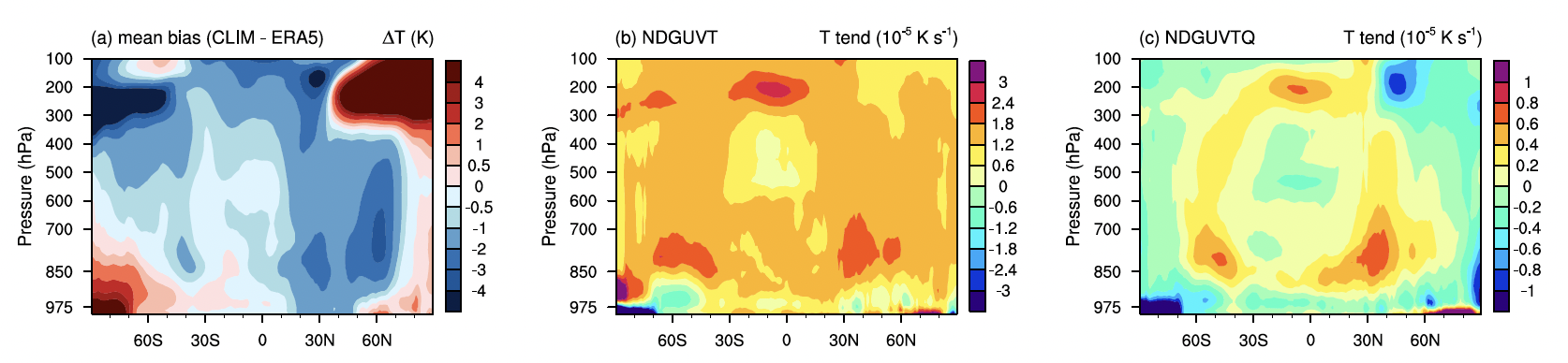
Figure 2 (a) monthly mean zonally averaged temperature differences (ΔT, unit: K) in January 2010 between ERA5 and EAM’s free-running simulation (CLIM in Table 1), (b-c) monthly mean nudging tendencies of temperature (T tend, unit K s−1) from the simulation by nudging EAM towards ERA5 reanalysis. The wind and temperature fields were nudged in the simulation (NDG_UVT in Tabel 1) for panel (b), while the wind, temperature and humidity were nudged in the simulation (NDG_UVTQ in Table 1) for panel (c). The y-axis of each panel shows the approximated pressure for the model levels in EAM.
Three groups of training data are generated in phase 1 (Table~ref{tabtrainning_exp}). The first group consists of the reference solution for U, V, T, Q that are derived from ERA5 reanalysis. The data are interpolated to the same grid and vertical levels for E3SM. The second group is a free-running baseline simulation referred to as CLIM. The before-radiation values of U, V, T, Q were archived to represent the baseline solution from the EAM-LR. The third group of simulations was nudged toward ERA5 reanalysis to derive the corrective tendencies of U, V, T, Q for ML training. The three pairs of simulation are conducted to construct an ensemble of training data sets by applying nudging:
to the horizontal winds with \(\tau\) = 6 (labeled “NDG_UV”)
to both winds and temperature with \(\tau\) = 6 (labeled “NDG_UVT”)
to winds, temperature, and humidity \(\tau\) = 6 (labeled “NDG_UVTQ”)

Table 1 List of reference data and EAM-LR simulations for machine learning. Note nudging is applied at every model physics time step (0.5-hr) for EAM.
All EAM simulations were conducted for 11-years from 2007 to 2017. The first year is for model spin-up and the remaining 10-years are used to construct the input data for ML training. Table 2 presents the list of the input variables for ML training. The 3-D model state (U, V, T, Q) variables are the instantaneous model output, while the nudging tendencies are averaged values during a 3-hr period for each time sample. The data are available at this [link]
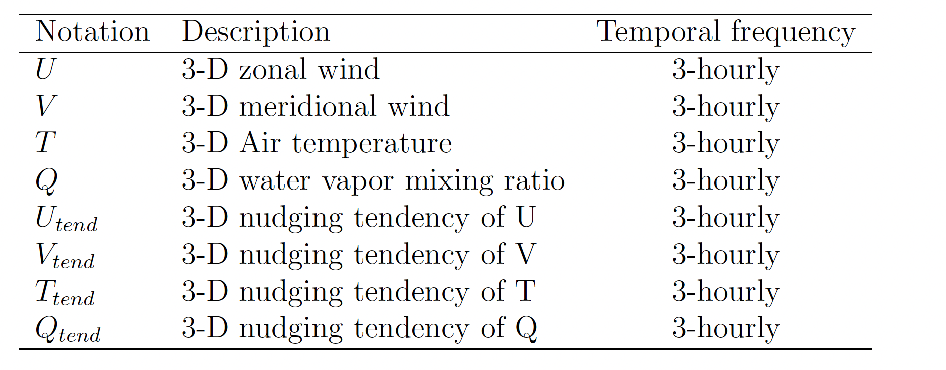
Table 2 Description of notation. Notes: the (x, y, z, t) is corresponding to the (latitude, logitude, levels, time) dimension in the EAM model output. Each notation contains the four state variables (i.e. U, V, T, Q) that are interested in this projec